
Ok… Since we decided to decode the C64 video signal, let’s start by recording the signal and having a look. The video signal is available on the A/V jack on the rear of the C64. Most C64 models have an 8-pin jack that provides separate luma (brightness) and chroma (color) signals on pins 1 and 6, and a composite video signal on pin 4. Some early models have a 5-pin jack that only provides luma and composite video.
The composite video signal is the sum of the luma and chroma signals, which is then modulated onto an RF carrier wave such that it can be connected to the antenna input of an analog TV. The composite video signal present on the A/V jack is the signal before RF modulation. Anway, since we want to examine the luma and chroma signals separately, we will take advantage of the separate signals. This way we don’t have to worry about splitting the composite video signal, nor the associated loss in signal quality. Should you happen to own a C64 with a 5-pin A/V jack, this means you will be stuck with black and white.
To record the luma and chroma signals, I used a Rigol DS1102E digital storage oscilloscope. With the scope’s memory depth set to “long”, the total number of samples the DS1102E can record is one mebisample, or 1048576 samples. When recording two channels simultaneously, the number of samples per channel is half this number.
There seems to be no way to set the sample rate of the scope directly. Instead, the sample rate is determined by the time scale used, in a rather obscure way. Some experimentation produced the table below, which for a given time scale gives the effective sample rate and the maximum recording duration (with “long” memory depth enabled). The duration was computed assuming two channels are being recorded at the same time. When recording a single channel, the maximum recording duration is twice that given in the table.
| Time scale | Duration (ms) | Sample rate (Ms/s) |
|---|---|---|
| 2 ns | 2.10 | 250 |
| 500 ns | 5.24 | 100 |
| 1 us | 5.24 | 100 |
| 2 us | 5.24 | 100 |
| 5 us | 5.24 | 100 |
| 10 us | 5.24 | 100 |
| 20 us | 5.24 | 100 |
| 50 us | 5.24 | 100 |
| 100 us | 5.24 | 100 |
| 200 us | 5.24 | 100 |
| 500 us | 10.49 | 50 |
| 1 ms | 26.21 | 20 |
| 2 ms | 52.43 | 10 |
| 10 ms | 262.14 | 2 |
The C64 generates approximately 50 video frames per second, so the duration of a single frame is 20 ms. To record both luma and chroma for a single frame, given the table above, the maximum sample rate we can achieve is 20 Ms/s (using a time scale of 1 ms).
To view the signals on the scope you can just connect the probes to pins 1 and 6 directly. This works fine. However, if you want to get the correct voltage levels, both signals should be terminated with a 75 ohm resistor to ground. Using a time scale of 1 ms, an a voltage scale of 500 mV, you should see something like the capture shown below. The amplitude of both signals should be 1 Vpp when properly terminated, which more or less agrees with the peak-to-peak voltages displayed on the scope.
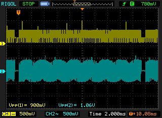
Captured video frame.
Luma is shown in yellow, chroma in blue. The traces have been shifted vertically so they don’t overlap. The gaps near the beginning and end of the luma trace are vertical synchronization pulses that mark the start (and end) of a frame. This confirms we have indeed captured a complete video frame.
For consistency, it would be nice to automatically trigger the recording at the start of a frame. The scope has a video trigger mode for exactly this purpose, but I couldn’t get it to work reliably with the C64 video signal. Luckily, Texas Instruments produces a video sync separator chip, the LM1881, which can still be found in a DIP package. It expects a composite video signal as input, but since it only relies on the synchronization pulses, we can simply feed it the luma signal. The LM1881 extracts various synchronization signals from the input signal. For the moment, we are only interested in the vertical synchronization signal, which is available on pin 3. This signal pulses low at the start of a frame.
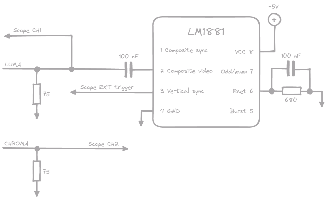
Circuit diagram of the acquisition setup.
The datasheet of the LM1881 provides a typical connection diagram, which I transferred to a breadboard. The only thing I added were termination resistors for the luma and chroma signal, and I used a variable resistor in place of the 680 ohm resistor to allow for fine-tuning should this be necessary. The cable coming in from the top of the image is connected to the C64 A/V jack. The brown wire carries the luma signal, the chroma signal is on the white wire. The luma signal is connected to the composite video input (pin 2) of the LM1881, and the vertical sync output (pin 3) is connected to the external trigger input of the scope. Luma is also connected to the first channel of the scope, and chroma to the second channel. Using this setup, the scope always starts recording at the start of a frame.
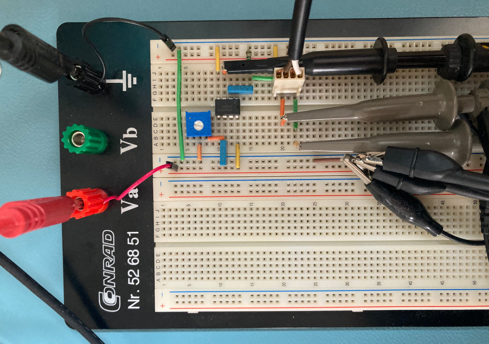
Setup used for acquisition.
Having found a way to reliably record video frames with the scope, the next step is to somehow retrieve the recorded samples. The Rigol has the ability to store recorded waveforms on a USB flash drive that you can plug into the connector on the front panel. This produces a file in Rigol’s proprietary WFM format. Several Python packages are available that can read these files. I used a small Python library by Matthias Blaicher.
While this works, repeatingly plugging a USB drive from the scope into the laptop and vice versa proved to be way too much hassle. Luckily for us, the Rigol scope has another USB connector on the rear panel that can be used to send it commands and retrieve recorded waveforms directly over USB. The protocol consists of simple ASCII commands. The Rigol Programming Guide contains a reference of all available commands. It can be found on the product page in the manual section.
The scope implements the USB test and measurement (usbtmc) device class. On
Linux, the kernel has built-in support for usbtmc devices. On my laptop, the
scope shows up as /dev/usbtmc0. Based on a blog post about
controlling a Rigol scope from Python, I created a small Python class to handle
the low-level I/O.
import os
import time

class RigolDSO:

    def __init__(self, device):

        self._device = device
        self._fd = None
        self._max_response_size = 4096 * 1024
        self._post_send_delay = 0.25

    def open(self):
        """Open the device."""
        assert self._fd is None
        self._fd = os.open(self._device, os.O_RDWR)

    def close(self):
        """Close the device."""
        if self._fd is not None:
            os.close(self._fd)
            self._fd = None

    def identity(self):
        """Get the scope's identification string."""
        return self.query("*IDN?")

    def reset(self):
        """Reset the scope."""
        self.send("*RST")
        time.sleep(2.0)

    def query_float(self, request):
        """Send an ASCII command to the oscilloscope; return the result as a float."""
        return float(self.query(request))

    def query(self, request):
        """Send an ASCII command to the oscilloscope; return the result as an ASCII string."""
        return self.query_raw(request).decode("ascii")

    def query_raw(self, request):
        """Send an ASCII command to the oscilloscope; return the result as raw bytes."""
        self.send(request)
        return os.read(self._fd, self._max_response_size)

    def send(self, request):
        """Send an ASCII string to the oscilloscope."""
        self.send_raw(request.encode("ascii"))
        time.sleep(self._post_send_delay)

    def send_raw(self, request):
        """Send raw bytes to the oscilloscope."""
        os.write(self._fd, request)

    def __enter__(self):
        """Context manager magic method; allows the device to be used in with statements."""
        self.open()
        return self

    def __exit__(self, exc_type, exc_value, exc_traceback):
        """Context manager magic method; allows the device to be used in with statements."""
        self.close()
Here is a small example Python script that uses this class to retrieve and print the scope’s identity string and some settings.
with RigolDSO("/dev/usbtmc0") as scope:

    print("Identity:", scope.identity())
    print("Time scale:", scope.query_float(":TIM:SCAL?"))
    print("Voltage scale (CH1):", scope.query_float(":CHAN1:SCAL?"))
    print("Voltage scale (CH2):", scope.query_float(":CHAN2:SCAL?"))
Now to record the video signal… All probes are assumed to be set to 10x attenuation. The probe for channel 1 should be connected to luma, channel 2 to chroma, and the external trigger input to the vertical sync output of the LM1881. The script below resets the scope such that we always start from the same settings. The memory depth is set to “long”, and the time scale is set to 1 ms. Channel 1 uses DC coupling (the default). The channel offset is set to shift the waveform downwards such that the 1 Vpp luma signal is nicely centered on the display. Channel 2 is set to use AC coupling. Unlike the luma signal, the chroma signal is a sinusoid (more or less), so AC coupling will take care of centering the waveform on the display. The external trigger is set to trigger on the falling edge of the LM1881 vertical sync output (the vertical sync output is active-low).
import matplotlib.pyplot as plt
import numpy as np

# Time scale in seconds.
dt = 1e-3

# Voltage scale in volts.
dV = 0.2

with RigolDSO("/dev/usbtmc0") as scope:

    # Reset the scope.
    scope.reset()

    # Set memory depth to long.
    scope.send(":ACQ:MEMD LONG")
    scope.send(":WAV:POINT:MODE RAW")

    # Set the time scale.
    scope.send(":TIM:SCAL {:.6f}".format(dt))

    # Configure channel 1 (luma).
    scope.send(":CHAN1:PROB 10")
    scope.send(":CHAN1:SCAL {:.6f}".format(dV))
    scope.send(":CHAN1:OFFS {:.6f}".format(-2 * dV))

    # Configure channel 2 (chroma).
    scope.send(":CHAN2:COUP AC")
    scope.send(":CHAN2:PROB 10")
    scope.send(":CHAN2:SCAL {:.6f}".format(dV))
    scope.send(":CHAN2:OFFS {:.6f}".format(0.0))

    # Configure the external trigger.
    scope.send(":TRIG:EDGE:SOUR EXT")
    scope.send(":TRIG:EDGE:SWE SING")
    scope.send(":TRIG:EDGE:SLOP NEG")
    scope.send(":TRIG:EDGE:LEV 0.5" )

    # Compute the waveform duration from the sample rate and set the time offset
    # to center the waveform in the display.
    sample_rate = scope.query_float(":ACQ:SAMP?")
    duration = (512 * 1024) / sample_rate
    scope.send(":TIM:OFFS {:.6f}".format(duration / 2.0))

    # Wait for a trigger.
    scope.send(":RUN")
    while scope.query(":TRIG:STAT?") != "STOP":
        time.sleep(0.5)
    scope.send(":STOP")

    # Retrieve the raw waveform data. Discard the first 10 bytes; these contain
    # unused header information.
    luma   = np.frombuffer(scope.query_raw(":WAV:DATA? CHAN1")[10:], np.uint8)
    chroma = np.frombuffer(scope.query_raw(":WAV:DATA? CHAN2")[10:], np.uint8)

plt.figure()
plt.title("Luma")
plt.ylabel("Luma (arbitrary unit)")
plt.xlabel("Time (ms)")
plt.plot(1e3 / sample_rate * np.arange(len(luma)), luma)

plt.figure()
plt.title("Chroma")
plt.ylabel("Chroma (arbitrary unit)")
plt.xlabel("Time (ms)")
plt.plot(1e3 / sample_rate * np.arange(len(chroma)), chroma)

for fignum in plt.get_fignums():

    figure = plt.figure(fignum)
    figure.canvas.mpl_connect("key_press_event", lambda event: plt.close("all"))

plt.show()
The script plots the recorded luma and chroma signals. The X-coordinate of each sample is a timestamp in milliseconds. The Y-coordinate is the raw sample value returned by the scope. Compared to the image of the scope display shown earlier, the luma signal is flipped vertically. (The chroma signal is also flipped, but that is harder to see since the signal is mostly symmetrical, so I did not show it here.)
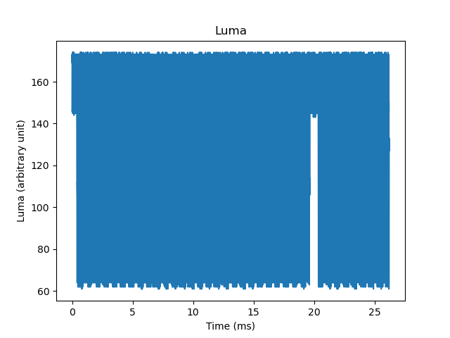
The raw luma signal retrieved from the scope.
So, what’s going on? Well… it turns out the raw sample values retrieved from the scope are Y-coordinates on the scope’s display. The Y-coordinate increases from top to bottom, while voltage increases from bottom to top, which is why the waveform appears to be upside-down.
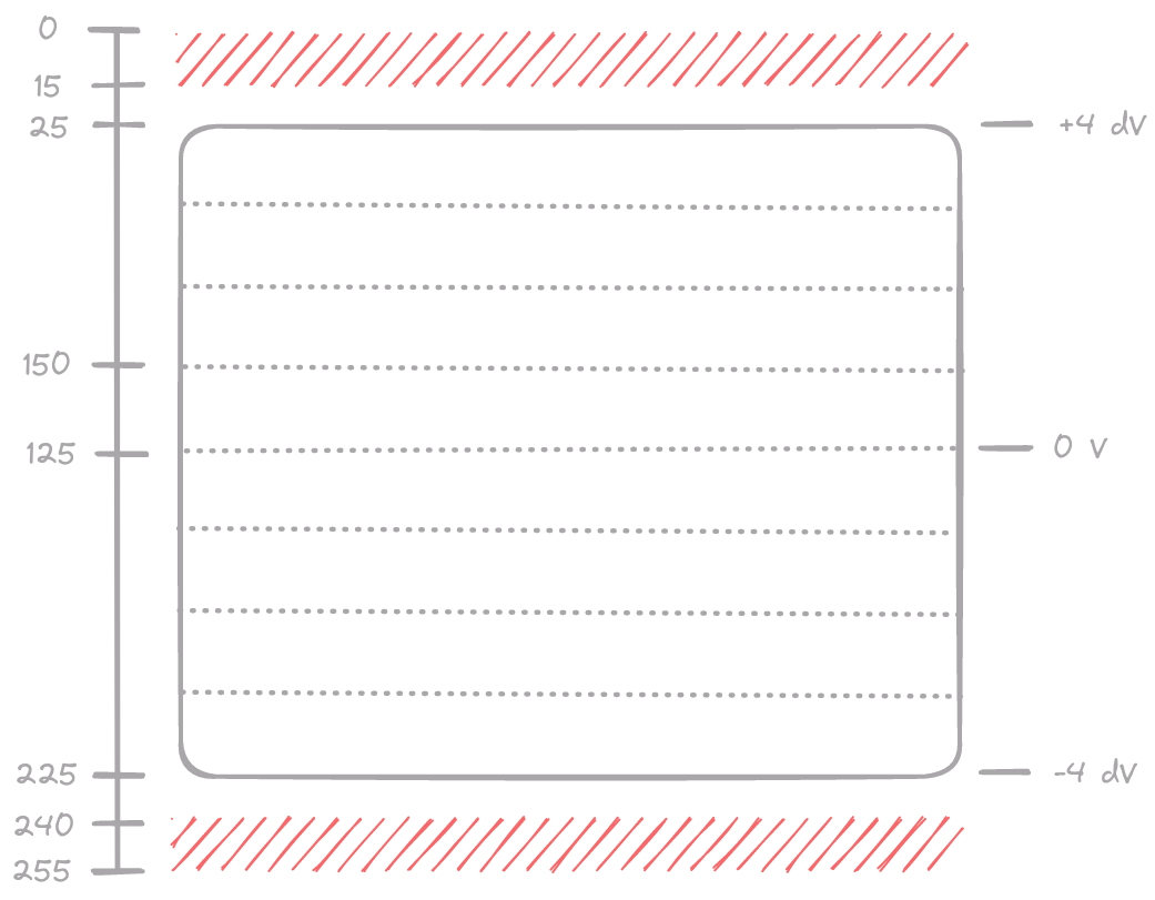
Scope display Y-coordinates.
Values smaller than 15 or larger than 240 never occur in the retrieved waveform data. This was found out by recording the luma signal with a suitably small voltage scale such that the signal extends well outside of the display. Values smaller than 25 or larger than 225 do occur, but are not visible on the display.
The Y-coordinate of the zero Volts line at the vertical center of the display seems to be 125. This value is the result of averaging several recordings with the probe attached to ground. A single voltage division is exactly 25 pixels high. There are 8 voltage divisions on the display, so the height of the display is 200 pixels. Using this information we can write a simple Python function to convert the raw waveform values to Volts.
def bytes_to_volts(raw_bytes, *, scale, offset):
    # The raw values returned by the scope are Y-coordinates on the scope's
    # display. The subset of the value range [0,255] that is visible on the
    # display is [25,225). The first visible Y-coordinate (25) represents the
    # top of the display.
    #
    # Zero volts is located at the center of the display, ie. at Y-coordinate
    # 25 + (225 - 25) / 2 = 125. If we subtract the raw values from 125, we get
    # signed "Y-coordinates" that are proportional to voltage.
    #
    # The height of the display is 225 - 25 = 200 pixels and contains 8 voltage
    # divisions. The voltage scale is given in Volts per division. So to convert
    # to volts, we have to divide by 200 / 8 = 25 to get (fractional, signed)
    # voltage divisions and then multiply by the voltage scale. Last but not
    # least, we correct for the voltage offset.
    return (125.0 - raw_bytes) / 25.0 * scale - offset
An important take-away from all of this is that to make the most of the available vertical resolution, we should choose a voltage scale and offset such that the signal we want to record covers as much of the display as possible without going outside of it. This is why a voltage scale of 0.2 V was used in the script, and an offset of -0.4 V was set for the luma channel.
UPDATE – I found a support article on the Rigol site that explains how to interpret the raw waveform data for the DS1052E/D oscilloscope. This model is very similar to the DS1102E. Expressed using the same variables as in the Python function above, the mapping from raw values to volts provided in this article is:
volts = (240.0 - raw_bytes) / 25.0 * scale - offset - 4.6 * scale
By hoisting the -4.6 * scale term inside the backets, this turns out to be
exactly equivalent to the mapping we reverse engineered.
volts = (125.0 - raw_bytes) / 25.0 * scale - offset
The article also confirms that values outside the range 15 – 240 do not occur, and that the range of values visible on the display is 25 – 225.
The actual script that I used for capturing luma and chroma signals is available
here. It has several command line options; run the script as
capture.py --help for an overview. For example, you can choose to record only
luma or only chroma at more than double the sampling rate (50 MHz instead of 20
MHz) or at 20 MHz for twice the duration. The script does not produce any
plots. Instead, the captured waveforms are stored as an HDF5 file for further
processing.
Speaking of further processing… In the next episode we will take a closer look at the luma signal and investigate how to turn it into an image.
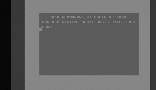
The Commodore BASIC screen in two shades of grey.